MNIST手写数字识别进阶
单隐藏层神经网络构建与应用
单个神经元模型
常见激活函数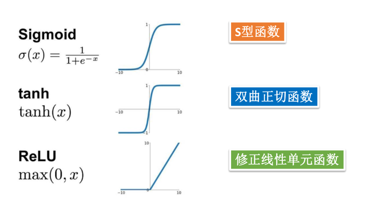
神经网络模型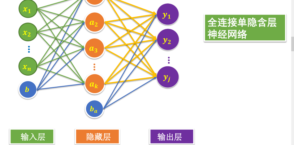
全连接单隐藏层网络建模实现
1.载入数据
2.构建输入层
·定义标签数据占位符
3.构建隐藏层1
2
3
4
5
6
7#隐藏层神经元数量
H1_MN = 256
W1 = tf.Variable(tf.random_normal([784,H1_MN]))
b1 = tf.Variable(tf.zeros([H1_MN]))
Y1 = tf.nn.relu(tf.matmul(x,W1) + b1)
4.构建输出层1
2
3
4
5W2 = tf.Variable(tf.random_normal([H1_MN,10]))
b2 = tf.Variable(tf.zeros([10]))
forward = tf.matmul(Y1,W2) + b2
pred = tf.nn.softmax(forward)
5.定义损失函数
6.训练模型
·设置训练参数
·选择优化器
·定义准确值
·记录训练开始时间
·读取批次数据
·执行批次训练
·验证数据计算误差与准确率
·显示运行时间
7.训练结果
8.评估模型
9.应用模型
·进行预测
·找出预测错误
·定义输出错误分类的函数
·可视化查看预测错误的样本
·定义可视化函数
完整程序如下:1
2
3
4
5
6
7
8
9
10
11
12
13
14
15
16
17
18
19
20
21
22
23
24
25
26
27
28
29
30
31
32
33
34
35
36
37
38
39
40
41
42
43
44
45
46
47
48
49
50
51
52
53
54
55
56
57
58
59
60
61
62
63
64
65
66
67
68
69
70
71
72
73
74
75
76
77
78
79
80
81
82
83
84
85
86
87
88
89
90
91
92
93
94
95
96
97
98
99
100
101
102
103
104
105
106
107
108
109
110
111
112
113
114
115
116
117
118
119
120import tensorflow as tf
import tensorflow.examples.tutorials.mnist.input_data as input_data
mnist = input_data.read_data_sets("MNIST_data/", one_hot=True)
x = tf.placeholder(tf.float32,[None, 784], name="X")
y = tf.placeholder(tf.float32,[None,10], name="Y")
H1_MN = 256
W1 = tf.Variable(tf.random_normal([784,H1_MN]))
b1 = tf.Variable(tf.zeros([H1_MN]))
Y1 = tf.nn.relu(tf.matmul(x,W1) + b1)
W2 = tf.Variable(tf.random_normal([H1_MN,10]))
b2 = tf.Variable(tf.zeros([10]))

forward = tf.matmul(Y1,W2) + b2
pred = tf.nn.softmax(forward)
loss_function = tf.reduce_mean(
tf.nn.softmax_cross_entropy_with_logits(logits=forward,labels=y))
train_epochs = 40
batch_size = 50
total_batch = int(mnist.train.num_examples/batch_size)
display_step = 1
learning_rate = 0.01
optimizer = tf.train.GradientDescentOptimizer(learning_rate).minimize(loss_function)
correct_prediction = tf.equal(tf.argmax(pred,1),tf.argmax(y,1))
accuracy = tf.reduce_mean(tf.cast(correct_prediction,tf.float32))
from time import time
startTime=time()
sess = tf.Session()
init = tf.global_variables_initializer()
sess.run(init)
for epoch in range (train_epochs):
for batch in range(total_batch):
xs,ys = mnist.train.next_batch(batch_size)
sess.run(optimizer,feed_dict={x:xs,y:ys})
loss,acc = sess.run([loss_function,accuracy],
feed_dict={x:mnist.validation.images,
y:mnist.validation.labels})
if(epoch+1) % display_step == 0:
print("Train Epoch:",'%02d' % (epoch+1),"Loss=","{:.9f}".format(loss),\
"Accuracy=","{:.4f}".format(acc))
duration = time() - startTime
print("Train Finshied takes:","{:.2f}".format(duration))
accu_test = sess.run(accuracy,
feed_dict={x:mnist.test.images,y:mnist.test.labels})
print("Test Accurary:",accu_test)
prediction_result = sess.run(tf.argmax(pred,1),
feed_dict = {x:mnist.test.images})
prediction_result[0:10]
import numpy as np
compare_lists = prediction_result==np.argmax(mnist.test.labels,1)
print(compare_lists)
err_lists = [i for i in range(len(compare_lists)) if compare_lists[i]==False]
print(err_lists, len(err_lists))
def print_predict_errs(labels,
prediction):
count = 0
compare_lists = (prediction==np.argmax(labels,1))
err_lists = [i for i in range(len(compare_lists)) if compare_lists[i]==False]
for x in err_lists:
print("index="+str(x)+
"标签值=",np.argmax(labels[x]),
"预测值=",prediction[x])
count = count + 1
print("总计:"+str(count))
print_predict_errs(labels=mnist.test.labels,
prediction=prediction_result)
import matplotlib.pyplot as plt
import numpy as np
def plot_images_labels_prediction(images,
labels,
prediction,
index,
num=10):
fig = plt.gcf()
fig.set_size_inches(10, 12)
if num > 25 :
num = 25
for i in range(0,num):
ax = plt.subplot(5,5,i+1)
ax.imshow(np.reshape(images[index],(28,28)),
cmap='binary')
title = "label=" + str(np.argmax(labels[index]))
if len(prediction)>0:
title += ",predict=" + str(prediction[index])
ax.set_title(title,fontsize=10)
ax.set_xticks([]);
ax.set_yticks([])
index += 1
plt.show()
plot_images_labels_prediction(mnist.test.images,
mnist.test.labels,
prediction_result,610,20)
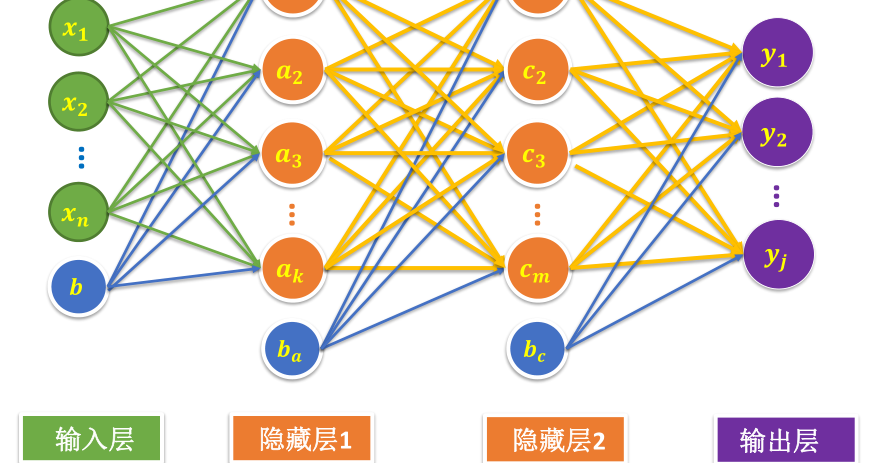
多层网络建模实现
1.构建模型1
2
3
4
5
6
7
8
9
10
11
12
13
14
15H1_MN = 256
H2_MN = 64
W1 = tf.Variable(tf.truncated_normal([784,H1_MN],stddev=0.1))
b1 = tf.Variable(tf.zeros([H1_MN]))
Y1 = tf.nn.relu(tf.matmul(x,W1) + b1)
W2 = tf.Variable(tf.truncated_normal([H1_MN,H2_MN],stddev=0.1))
b2 = tf.Variable(tf.zeros([H2_MN]))
Y2 = tf.nn.relu(tf.matmul(Y1,W2) + b2)
W3 = tf.Variable(tf.truncated_normal([H2_MN,10],stddev=0.1))
b3 = tf.Variable(tf.zeros([10]))
其余程序与步骤都相同
完整程序如下:1
2
3
4
5
6
7
8
9
10
11
12
13
14
15
16
17
18
19
20
21
22
23
24
25
26
27
28
29
30
31
32
33
34
35
36
37
38
39
40
41
42
43
44
45
46
47
48
49
50
51
52
53
54
55
56
57
58
59
60
61
62
63
64
65
66
67
68
69
70
71
72
73
74
75
76
77
78
79
80
81
82
83
84
85
86
87
88
89
90
91
92
93
94
95
96
97
98
99
100
101
102
103
104
105
106
107
108
109
110
111
112
113
114
115
116
117
118
119
120
121
122
123
124
125
126import tensorflow as tf
import tensorflow.examples.tutorials.mnist.input_data as input_data
mnist = input_data.read_data_sets("MNIST_data/", one_hot=True)
x = tf.placeholder(tf.float32,[None, 784], name="X")
y = tf.placeholder(tf.float32,[None,10], name="Y")
H1_MN = 256
H2_MN = 64

W1 = tf.Variable(tf.truncated_normal([784,H1_MN],stddev=0.1))
b1 = tf.Variable(tf.zeros([H1_MN]))

Y1 = tf.nn.relu(tf.matmul(x,W1) + b1)

W2 = tf.Variable(tf.truncated_normal([H1_MN,H2_MN],stddev=0.1))
b2 = tf.Variable(tf.zeros([H2_MN]))

Y2 = tf.nn.relu(tf.matmul(Y1,W2) + b2)

W3 = tf.Variable(tf.truncated_normal([H2_MN,10],stddev=0.1))
b3 = tf.Variable(tf.zeros([10]))
forward = tf.matmul(Y2,W3) + b3
pred = tf.nn.softmax(forward)
loss_function = tf.reduce_mean(
tf.nn.softmax_cross_entropy_with_logits(logits=forward,labels=y))
train_epochs = 40
batch_size = 50
total_batch = int(mnist.train.num_examples/batch_size)
display_step = 1
learning_rate = 0.01
optimizer = tf.train.GradientDescentOptimizer(learning_rate).minimize(loss_function)
correct_prediction = tf.equal(tf.argmax(pred,1),tf.argmax(y,1))
accuracy = tf.reduce_mean(tf.cast(correct_prediction,tf.float32))
from time import time
startTime=time()
sess = tf.Session()
init = tf.global_variables_initializer()
sess.run(init)
for epoch in range (train_epochs):
for batch in range(total_batch):
xs,ys = mnist.train.next_batch(batch_size)
sess.run(optimizer,feed_dict={x:xs,y:ys})
loss,acc = sess.run([loss_function,accuracy],
feed_dict={x:mnist.validation.images,
y:mnist.validation.labels})
if(epoch+1) % display_step == 0:
print("Train Epoch:",'%02d' % (epoch+1),"Loss=","{:.9f}".format(loss),\
"Accuracy=","{:.4f}".format(acc))
duration = time() - startTime
print("Train Finshied takes:","{:.2f}".format(duration))
accu_test = sess.run(accuracy,
feed_dict={x:mnist.test.images,y:mnist.test.labels})
print("Test Accurary:",accu_test)
prediction_result = sess.run(tf.argmax(pred,1),
feed_dict = {x:mnist.test.images})
prediction_result[0:10]
import numpy as np
compare_lists = prediction_result==np.argmax(mnist.test.labels,1)
print(compare_lists)
err_lists = [i for i in range(len(compare_lists)) if compare_lists[i]==False]
print(err_lists, len(err_lists))
def print_predict_errs(labels,
prediction):
count = 0
compare_lists = (prediction==np.argmax(labels,1))
err_lists = [i for i in range(len(compare_lists)) if compare_lists[i]==False]
for x in err_lists:
print("index="+str(x)+
"标签值=",np.argmax(labels[x]),
"预测值=",prediction[x])
count = count + 1
print("总计:"+str(count))
print_predict_errs(labels=mnist.test.labels,
prediction=prediction_result)
import matplotlib.pyplot as plt
import numpy as np
def plot_images_labels_prediction(images,
labels,
prediction,
index,
num=10):
fig = plt.gcf()
fig.set_size_inches(10, 12)
if num > 25 :
num = 25
for i in range(0,num):
ax = plt.subplot(5,5,i+1)
ax.imshow(np.reshape(images[index],(28,28)),
cmap='binary')
title = "label=" + str(np.argmax(labels[index]))
if len(prediction)>0:
title += ",predict=" + str(prediction[index])
ax.set_title(title,fontsize=10)
ax.set_xticks([]);
ax.set_yticks([])
index += 1
plt.show()
plot_images_labels_prediction(mnist.test.images,
mnist.test.labels,
prediction_result,610,20)
训练结果如下显示:(多数据警告)
Train Epoch: 01 Loss= 0.420293599 Accuracy= 0.8820
Train Epoch: 02 Loss= 0.314055026 Accuracy= 0.9136
Train Epoch: 03 Loss= 0.270856827 Accuracy= 0.9234
Train Epoch: 04 Loss= 0.241648629 Accuracy= 0.9310
Train Epoch: 05 Loss= 0.221271217 Accuracy= 0.9378
Train Epoch: 06 Loss= 0.202354938 Accuracy= 0.9440
Train Epoch: 07 Loss= 0.190346196 Accuracy= 0.9464
Train Epoch: 08 Loss= 0.176857352 Accuracy= 0.9516
Train Epoch: 09 Loss= 0.166498899 Accuracy= 0.9536
Train Epoch: 10 Loss= 0.157787085 Accuracy= 0.9546
Train Epoch: 11 Loss= 0.153465509 Accuracy= 0.9576
Train Epoch: 12 Loss= 0.143812209 Accuracy= 0.9608
Train Epoch: 13 Loss= 0.140448615 Accuracy= 0.9594
Train Epoch: 14 Loss= 0.134099528 Accuracy= 0.9630
Train Epoch: 15 Loss= 0.132911429 Accuracy= 0.9624
Train Epoch: 16 Loss= 0.124732591 Accuracy= 0.9660
Train Epoch: 17 Loss= 0.119741030 Accuracy= 0.9672
Train Epoch: 18 Loss= 0.120224647 Accuracy= 0.9648
Train Epoch: 19 Loss= 0.114067823 Accuracy= 0.9676
Train Epoch: 20 Loss= 0.111958325 Accuracy= 0.9684
Train Epoch: 21 Loss= 0.111831568 Accuracy= 0.9672
Train Epoch: 22 Loss= 0.106434591 Accuracy= 0.9700
Train Epoch: 23 Loss= 0.105766617 Accuracy= 0.9688
Train Epoch: 24 Loss= 0.102649413 Accuracy= 0.9710
Train Epoch: 25 Loss= 0.101922378 Accuracy= 0.9712
Train Epoch: 26 Loss= 0.100112967 Accuracy= 0.9708
Train Epoch: 27 Loss= 0.096768998 Accuracy= 0.9724
Train Epoch: 28 Loss= 0.097221516 Accuracy= 0.9732
Train Epoch: 29 Loss= 0.095773250 Accuracy= 0.9726
Train Epoch: 30 Loss= 0.094824158 Accuracy= 0.9734
Train Epoch: 31 Loss= 0.092812546 Accuracy= 0.9734
Train Epoch: 32 Loss= 0.092194885 Accuracy= 0.9736
Train Epoch: 33 Loss= 0.090828940 Accuracy= 0.9746
Train Epoch: 34 Loss= 0.088991299 Accuracy= 0.9748
Train Epoch: 35 Loss= 0.089945436 Accuracy= 0.9750
Train Epoch: 36 Loss= 0.086703502 Accuracy= 0.9762
Train Epoch: 37 Loss= 0.087226808 Accuracy= 0.9758
Train Epoch: 38 Loss= 0.086025327 Accuracy= 0.9758
Train Epoch: 39 Loss= 0.085212491 Accuracy= 0.9758
Train Epoch: 40 Loss= 0.085250698 Accuracy= 0.9762
Train Finshied takes: 94.00
Test Accurary: 0.9727
[ True True True … True True True]
[8, 104, 247, 259, 320, 340, 381, 445, 449, 495, 582, 610, 613, 659, 684, 691, 707, 720, 740, 810, 813, 844, 890, 938, 951, 956, 959, 965, 982, 1014, 1032, 1039, 1107, 1112, 1114, 1156, 1181, 1182, 1192, 1194, 1224, 1226, 1232, 1242, 1247, 1260, 1319, 1326, 1328, 1378, 1393, 1444, 1500, 1522, 1527, 1530, 1549, 1553, 1570, 1609, 1621, 1671, 1681, 1717, 1754, 1790, 1800, 1850, 1878, 1901, 1911, 1913, 1940, 1941, 1984, 2016, 2035, 2044, 2053, 2070, 2109, 2118, 2129, 2130, 2135, 2145, 2182, 2186, 2195, 2224, 2266, 2272, 2280, 2293, 2333, 2369, 2387, 2406, 2414, 2433, 2455, 2488, 2514, 2573, 2607, 2618, 2648, 2654, 2721, 2863, 2877, 2896, 2915, 2939, 2953, 2979, 2995, 3005, 3030, 3060, 3073, 3117, 3405, 3422, 3503, 3520, 3533, 3549, 3558, 3567, 3575, 3597, 3718, 3751, 3767, 3776, 3780, 3796, 3808, 3811, 3838, 3846, 3853, 3869, 3893, 3902, 3906, 3929, 3941, 3946, 3968, 3985, 3995, 4007, 4065, 4075, 4078, 4163, 4177, 4201, 4211, 4224, 4248, 4289, 4306, 4374, 4437, 4451, 4477, 4497, 4534, 4536, 4578, 4601, 4635, 4668, 4761, 4807, 4814, 4823, 4860, 4874, 4876, 4880, 4956, 4966, 5078, 5265, 5331, 5457, 5600, 5642, 5676, 5734, 5749, 5887, 5936, 5937, 5955, 5973, 5982, 5997, 6023, 6045, 6046, 6059, 6071, 6101, 6166, 6173, 6390, 6400, 6426, 6505, 6532, 6557, 6560, 6571, 6590, 6597, 6608, 6625, 6651, 6783, 6847, 7434, 7451, 7595, 7800, 7821, 7849, 7858, 7886, 7899, 7915, 7991, 8062, 8094, 8272, 8277, 8311, 8325, 8339, 8408, 8520, 8522, 9009, 9015, 9019, 9024, 9071, 9280, 9482, 9587, 9634, 9636, 9662, 9692, 9698, 9729, 9745, 9749, 9768, 9770, 9779, 9811, 9828, 9839, 9879, 9888, 9891, 9944, 9982] 273
index=8标签值= 5 预测值= 6
index=104标签值= 9 预测值= 5
index=247标签值= 4 预测值= 6
index=259标签值= 6 预测值= 0
index=320标签值= 9 预测值= 8
index=340标签值= 5 预测值= 3
index=381标签值= 3 预测值= 7
index=445标签值= 6 预测值= 0
index=449标签值= 3 预测值= 5
index=495标签值= 8 预测值= 2
index=582标签值= 8 预测值= 2
index=610标签值= 4 预测值= 2
index=613标签值= 2 预测值= 8
index=659标签值= 2 预测值= 8
index=684标签值= 7 预测值= 3
index=691标签值= 8 预测值= 4
index=707标签值= 4 预测值= 9
index=720标签值= 5 预测值= 8
index=740标签值= 4 预测值= 9
index=810标签值= 7 预测值= 2
index=813标签值= 9 预测值= 8
index=844标签值= 8 预测值= 7
index=890标签值= 3 预测值= 5
index=938标签值= 3 预测值= 5
index=951标签值= 5 预测值= 4
index=956标签值= 1 预测值= 2
index=959标签值= 4 预测值= 9
index=965标签值= 6 预测值= 0
index=982标签值= 3 预测值= 2
index=1014标签值= 6 预测值= 5
index=1032标签值= 5 预测值= 8
index=1039标签值= 7 预测值= 8
index=1107标签值= 9 预测值= 5
index=1112标签值= 4 预测值= 6
index=1114标签值= 3 预测值= 8
index=1156标签值= 7 预测值= 8
index=1181标签值= 6 预测值= 1
index=1182标签值= 6 预测值= 8
index=1192标签值= 9 预测值= 4
index=1194标签值= 7 预测值= 9
index=1224标签值= 2 预测值= 6
index=1226标签值= 7 预测值= 2
index=1232标签值= 9 预测值= 4
index=1242标签值= 4 预测值= 9
index=1247标签值= 9 预测值= 5
index=1260标签值= 7 预测值= 1
index=1319标签值= 8 预测值= 3
index=1326标签值= 7 预测值= 2
index=1328标签值= 7 预测值= 8
index=1378标签值= 5 预测值= 6
index=1393标签值= 5 预测值= 3
index=1444标签值= 6 预测值= 4
index=1500标签值= 7 预测值= 1
index=1522标签值= 7 预测值= 9
index=1527标签值= 1 预测值= 6
index=1530标签值= 8 预测值= 7
index=1549标签值= 4 预测值= 2
index=1553标签值= 9 预测值= 3
index=1570标签值= 0 预测值= 6
index=1609标签值= 2 预测值= 6
index=1621标签值= 0 预测值= 6
index=1671标签值= 7 预测值= 3
index=1681标签值= 3 预测值= 7
index=1717标签值= 8 预测值= 0
index=1754标签值= 7 预测值= 2
index=1790标签值= 2 预测值= 8
index=1800标签值= 6 预测值= 4
index=1850标签值= 8 预测值= 3
index=1878标签值= 8 预测值= 3
index=1901标签值= 9 预测值= 4
index=1911标签值= 5 预测值= 6
index=1913标签值= 3 预测值= 8
index=1940标签值= 5 预测值= 0
index=1941标签值= 7 预测值= 8
index=1984标签值= 2 预测值= 0
index=2016标签值= 7 预测值= 2
index=2035标签值= 5 预测值= 3
index=2044标签值= 2 预测值= 7
index=2053标签值= 4 预测值= 9
index=2070标签值= 7 预测值= 9
index=2109标签值= 3 预测值= 9
index=2118标签值= 6 预测值= 1
index=2129标签值= 9 预测值= 2
index=2130标签值= 4 预测值= 9
index=2135标签值= 6 预测值= 1
index=2145标签值= 4 预测值= 2
index=2182标签值= 1 预测值= 2
index=2186标签值= 2 预测值= 3
index=2195标签值= 7 预测值= 2
index=2224标签值= 5 预测值= 8
index=2266标签值= 1 预测值= 8
index=2272标签值= 8 预测值= 0
index=2280标签值= 3 预测值= 5
index=2293标签值= 9 预测值= 6
index=2333标签值= 0 预测值= 2
index=2369标签值= 5 预测值= 8
index=2387标签值= 9 预测值= 1
index=2406标签值= 9 预测值= 1
index=2414标签值= 9 预测值= 4
index=2433标签值= 2 预测值= 1
index=2455标签值= 0 预测值= 6
index=2488标签值= 2 预测值= 4
index=2514标签值= 4 预测值= 9
index=2573标签值= 5 预测值= 8
index=2607标签值= 7 预测值= 1
index=2618标签值= 3 预测值= 5
index=2648标签值= 9 预测值= 0
index=2654标签值= 6 预测值= 1
index=2721标签值= 6 预测值= 5
index=2863标签值= 9 预测值= 4
index=2877标签值= 4 预测值= 7
index=2896标签值= 8 预测值= 0
index=2915标签值= 7 预测值= 3
index=2939标签值= 9 预测值= 5
index=2953标签值= 3 预测值= 5
index=2979标签值= 9 预测值= 7
index=2995标签值= 6 预测值= 5
index=3005标签值= 9 预测值= 1
index=3030标签值= 6 预测值= 2
index=3060标签值= 9 预测值= 7
index=3073标签值= 1 预测值= 3
index=3117标签值= 5 预测值= 9
index=3405标签值= 4 预测值= 9
index=3422标签值= 6 预测值= 0
index=3503标签值= 9 预测值= 1
index=3520标签值= 6 预测值= 4
index=3533标签值= 4 预测值= 9
index=3549标签值= 3 预测值= 2
index=3558标签值= 5 预测值= 0
index=3567标签值= 8 预测值= 5
index=3575标签值= 7 预测值= 8
index=3597标签值= 9 预测值= 3
index=3718标签值= 4 预测值= 9
index=3751标签值= 7 预测值= 2
index=3767标签值= 7 预测值= 3
index=3776标签值= 5 预测值= 8
index=3780标签值= 4 预测值= 6
index=3796标签值= 2 预测值= 8
index=3808标签值= 7 预测值= 8
index=3811标签值= 2 预测值= 0
index=3838标签值= 7 预测值= 1
index=3846标签值= 6 预测值= 4
index=3853标签值= 6 预测值= 2
index=3869标签值= 9 预测值= 4
index=3893标签值= 5 预测值= 6
index=3902标签值= 5 预测值= 3
index=3906标签值= 1 预测值= 3
index=3929标签值= 5 预测值= 8
index=3941标签值= 4 预测值= 2
index=3946标签值= 2 预测值= 8
index=3968标签值= 5 预测值= 3
index=3985标签值= 9 预测值= 4
index=3995标签值= 3 预测值= 5
index=4007标签值= 7 预测值= 4
index=4065标签值= 0 预测值= 7
index=4075标签值= 8 预测值= 0
index=4078标签值= 9 预测值= 3
index=4163标签值= 9 预测值= 0
index=4177标签值= 5 预测值= 4
index=4201标签值= 1 预测值= 7
index=4211标签值= 6 预测值= 5
index=4224标签值= 9 预测值= 7
index=4248标签值= 2 预测值= 8
index=4289标签值= 2 预测值= 8
index=4306标签值= 3 预测值= 7
index=4374标签值= 5 预测值= 6
index=4437标签值= 3 预测值= 2
index=4451标签值= 2 预测值= 8
index=4477标签值= 0 预测值= 6
index=4497标签值= 8 预测值= 2
index=4534标签值= 9 预测值= 8
index=4536标签值= 6 预测值= 5
index=4578标签值= 7 预测值= 9
index=4601标签值= 8 预测值= 4
index=4635标签值= 3 预测值= 5
index=4668标签值= 2 预测值= 3
index=4761标签值= 9 预测值= 8
index=4807标签值= 8 预测值= 3
index=4814标签值= 6 预测值= 0
index=4823标签值= 9 预测值= 4
index=4860标签值= 4 预测值= 9
index=4874标签值= 9 预测值= 6
index=4876标签值= 2 预测值= 4
index=4880标签值= 0 预测值= 8
index=4956标签值= 8 预测值= 4
index=4966标签值= 7 预测值= 3
index=5078标签值= 3 预测值= 8
index=5265标签值= 6 预测值= 4
index=5331标签值= 1 预测值= 6
index=5457标签值= 1 预测值= 8
index=5600标签值= 7 预测值= 9
index=5642标签值= 1 预测值= 8
index=5676标签值= 4 预测值= 3
index=5734标签值= 3 预测值= 2
index=5749标签值= 8 预测值= 6
index=5887标签值= 7 预测值= 0
index=5936标签值= 4 预测值= 9
index=5937标签值= 5 预测值= 3
index=5955标签值= 3 预测值= 8
index=5973标签值= 3 预测值= 8
index=5982标签值= 5 预测值= 3
index=5997标签值= 5 预测值= 8
index=6023标签值= 3 预测值= 8
index=6045标签值= 3 预测值= 9
index=6046标签值= 3 预测值= 8
index=6059标签值= 3 预测值= 9
index=6071标签值= 9 预测值= 3
index=6101标签值= 1 预测值= 8
index=6166标签值= 9 预测值= 3
index=6173标签值= 9 预测值= 0
index=6390标签值= 5 预测值= 8
index=6400标签值= 0 预测值= 6
index=6426标签值= 0 预测值= 6
index=6505标签值= 9 预测值= 0
index=6532标签值= 0 预测值= 5
index=6557标签值= 0 预测值= 2
index=6560标签值= 9 预测值= 3
index=6571标签值= 9 预测值= 7
index=6590标签值= 0 预测值= 5
index=6597标签值= 0 预测值= 7
index=6608标签值= 9 预测值= 5
index=6625标签值= 8 预测值= 2
index=6651标签值= 0 预测值= 5
index=6783标签值= 1 预测值= 6
index=6847标签值= 6 预测值= 4
index=7434标签值= 4 预测值= 8
index=7451标签值= 5 预测值= 6
index=7595标签值= 3 预测值= 8
index=7800标签值= 3 预测值= 2
index=7821标签值= 3 预测值= 2
index=7849标签值= 3 预测值= 2
index=7858标签值= 3 预测值= 2
index=7886标签值= 2 预测值= 4
index=7899标签值= 1 预测值= 8
index=7915标签值= 7 预测值= 8
index=7991标签值= 9 预测值= 8
index=8062标签值= 5 预测值= 8
index=8094标签值= 2 预测值= 8
index=8272标签值= 3 预测值= 5
index=8277标签值= 3 预测值= 8
index=8311标签值= 6 预测值= 4
index=8325标签值= 0 预测值= 6
index=8339标签值= 8 预测值= 6
index=8408标签值= 8 预测值= 6
index=8520标签值= 4 预测值= 8
index=8522标签值= 8 预测值= 6
index=9009标签值= 7 预测值= 2
index=9015标签值= 7 预测值= 2
index=9019标签值= 7 预测值= 2
index=9024标签值= 7 预测值= 2
index=9071标签值= 1 预测值= 8
index=9280标签值= 8 预测值= 5
index=9482标签值= 5 预测值= 3
index=9587标签值= 9 预测值= 4
index=9634标签值= 0 预测值= 8
index=9636标签值= 3 预测值= 5
index=9662标签值= 3 预测值= 2
index=9692标签值= 9 预测值= 7
index=9698标签值= 6 预测值= 5
index=9729标签值= 5 预测值= 6
index=9745标签值= 4 预测值= 2
index=9749标签值= 5 预测值= 6
index=9768标签值= 2 预测值= 0
index=9770标签值= 5 预测值= 0
index=9779标签值= 2 预测值= 0
index=9811标签值= 2 预测值= 8
index=9828标签值= 3 预测值= 5
index=9839标签值= 2 预测值= 7
index=9879标签值= 0 预测值= 2
index=9888标签值= 6 预测值= 0
index=9891标签值= 9 预测值= 7
index=9944标签值= 3 预测值= 8
index=9982标签值= 5 预测值= 6
总计:273
此外我又尝试了两层隐藏网络的模型效果,事实上网络层数并不是越多越好,在这里不再赘述
重构建模过程
构建模型
·定义隐藏层神经元数目
·输入层:隐藏层参数和偏置项
·计算隐藏层结果
·计算输出结果
新定义全连接层函数1
2
3
4
5
6
7
8
9
10
11
12
13
14
15
16def fcn_layer(inputs,
input_dim,
output_dim,
activation=None):
W = tf.Variable(tf.truncated_normal([input_dim,output_dim],stddve=0.1))
b = tf.Variable(tf.zeros([output_dim]))
XWb = tf.matmul(inputs, W) + b
if activation is None:
outputs = XWb
else:
outputs = activation(XWb)
return outputs
·构建输入层
·构建隐藏层(1…n)
·构建输出层
训练模型的保存
初始化参数和文件目录1
2
3
4
5
6
7
8
9
10
11
12
13
14
15
16
17
18
19#存储模型的粒度
save = 5
#创建保存模型文件的目录
import os
ckpt_dir = "./ckpt_dir"
if not os.path.exists(ckpt_dir):
os.makedirs(ckpt_dir)
saver = tf.train.Saver()
if(epoch+1) % save_step == 0:
saver.save(sess, os.path.join(ckpt_dir,
'mnist_h256_model_{:06d}.ckpt'.format(epoch+1)))#存储模型
print('mnist_h256_model_{:06d}.ckpt saved'.format(epoch+1))
saver.save(sess, os.path.join(ckpt_dir,'mnist_h256_model.ckpt'))
print("Model saved!")
训练模型的还原与应用
1.定义相同结构的模型
2.设置模型文件的存放目录
3.读取还原模型1
2
3
4
5
6
7
8
9
10saver = tf.train. Saver()
sess = tf.Session()
init = tf.global_variables_initializer()
sess.run(init)
ckpt = tf.train. get_checkpoint_state(ckpt_dir)
if ckpt and ckpt.model_checkpoint_path:
saver. restore(sess,ckpt.model_checkpoint_path)#从已保存的模型中读取参数
print("Restore model from "+ckpt.model_checkpoint_path)
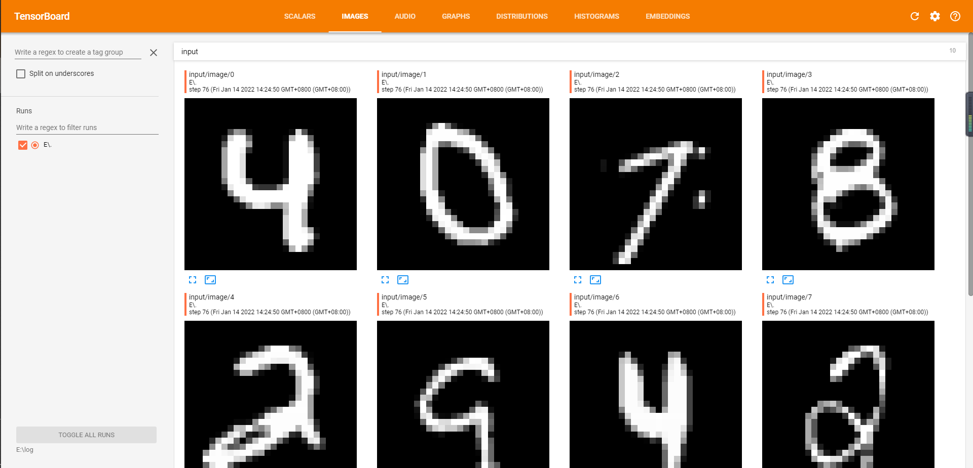
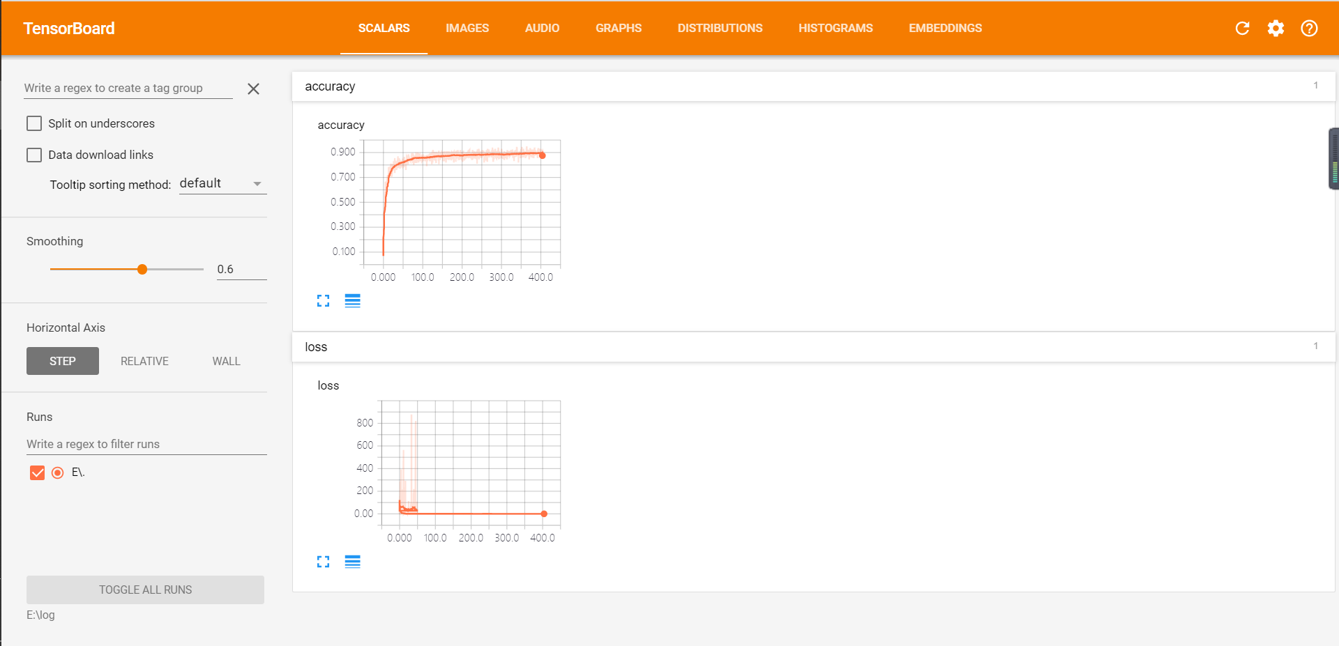
TensorBoard进阶与Tensorflow游乐场
TensorBoard进阶
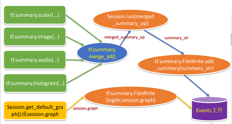
1 | image_shaped_input = tf.reshape(x, [-1,28,28,1]) |
启动tensorboard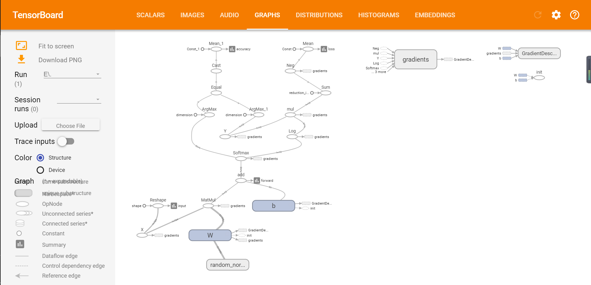
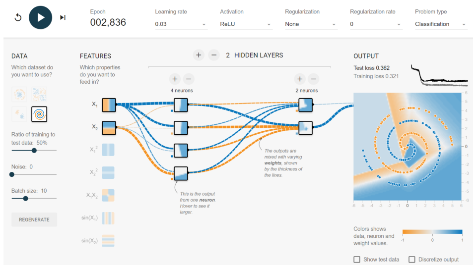
Tensorflow游乐场
TensorFlow游乐场是一个通过网页浏览器就可以训练的简单神经网络并实现了可视化训练过程
网址:http://playground.tensorflow.org
数据
每个点代表一个样本
点的颜色代表样本标签
提供了4种不同的数据集,可以设置训练数据比例、噪音、批处理大小
特征提取
为了将一个实际问题对应到平面上不同颜色点的划分,需要将实际问题种的实体变成平面上的一个点;点的颜色只有两种,这是一个二分类的问题
以判断零件是否合格为例,长度和质量就是特征
在机器学习中,所有用于描述实体的数字的组合就是一个实体的特征向量(feature vector)
神经网络
神经网络是分层的机构
特征向量是神经网络的输入层
同一层的节点不会互相连接
每一层只和下一层连接
最后一层作为输出层得到结果
输入和输出层之间的是隐藏层
学习率(learning rate)、激活函数(activation)、正则化(regularization)
神经网络训练解读
一个小格子代表神经网络中的一个节点
边代表节点之间的连接
节点和边都有或深或浅的颜色
边代表了神经网络的一个参数,可以是任意实数
神经网络就是通过对参数的合理设置来解决分类或者回归问题的
边的颜色体现了这个参数的取值,颜色越深,绝对值越大
节点的颜色代表了区分平面。这个平面上的每个点就代表了(x1,x2)的一种取值,当节点的输出值的绝对值越大时,颜色越深(蓝色)
例:x1节点的区分平面就是y轴
输出节点除了显示区分平面外,还显示了训练数据