卷积神经网络Convolutional Neural Network(CNN)
图像分类
ImageNet图像分类错误率(top-5)当卷积神经网络达到152层时,错误率可达到3.57.而同比人类的错误率为5.1
卷积神经网络成了机器视觉任务的一个极为重要的工具!
认识卷积神经网络-TensorFlow对卷积神经网络的支持-案例:CIFAR-10图像识别
从全连接神经网络到卷积神经网络
全连接网络的局限性
对于MNIST 手写数字识别,假如第一个隐层的节点数为500,那么一个全连接层的参数个数为:
28×28×1×500+500 ≈ 40万;
当图片更大时,比如CIFAR数据集中,图片大小为32×32×3,此时全连接层的参数有:
32×32×3×500+500 ≈ 150万
当图片分辨率进一步提高时,当隐层数量增加时,
例如:600 x 600 图像,各隐层节点数分别为300,200和100,则参数个数为:
600 x 600 x 300 + 300 x 200 + 200 x 100 ≈ 1.08亿
参数增多会导致:
计算速度减慢
过拟合
需要更合理的结构来有效减少参数个数
卷积神经网络的提出
1962年Hubel和Wiesel通过对猫视觉皮层细胞的研究,提出了感受野(receptive field)的概念。视觉皮层的神经元就是局部接受信息的,只受某些特定区域刺激的响应,而不是对全局图像进行感知。
1984年日本学者Fukushima基于感受野概念提出神经认知机(neocognitron)。
CNN可看作是神经认知机的推广形式。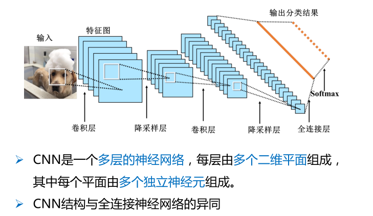
卷积
在介绍卷积神经网络的基本概念之前,我们先做一个矩阵运算:
(1)求点积:将5×5输入矩阵中3×3深蓝色区域中每个元素分别与其对应位置的权值(红色数字)相乘,然后再相加,所得到的值作为3×3输出矩阵(绿色)的第一个元素。
(2)滑动窗口:将3×3权值矩阵向右移动一个格(即,步长为1)
(3)重复操作:同样地,将此时深色区域内每个元素分别与对应的权值相乘然后再相加,所得到的值作为输出矩阵的第二个元素;重复上述“求点积-滑动窗口”操作,直至输出矩阵所有值被填满。
卷积核在 2 维输入数据上“滑动”,对当前输入部分的元素进行矩阵乘法,然后将结果汇为单个输出像素值,重复这个过程直到遍历整张图像,这个过程就叫做卷积,这个权值矩阵就是卷积核
卷积操作后的图像称为特征图(feature map)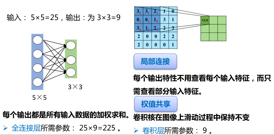
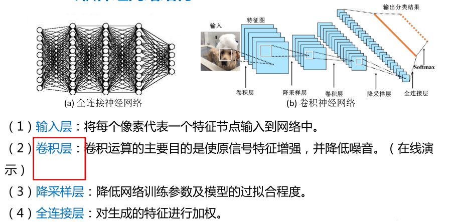
卷积层:卷积运算的主要目的是使原信号特征增强,并降低噪音。
定义卷积核 → 卷积操作 → 显示
卷积运算的主要目的是使原信号特征增强,并降低噪音。
对图像用一个卷积核进行卷积运算,实际上是一个滤波的过程。每个卷积核都是一种特征提取方式,就像是一个筛子,将图像中符合条件的部分筛选出来。
0填充(Padding)
观察卷积示例,我们会发现一个现象:在卷积核滑动的过程中图像的边缘会被裁剪掉,将5×5特征矩阵转换为 3×3的特征矩阵。
如何使得输出尺寸与输入保持一致呢?
0填充:
用额外的“假”像素(通常值为 0)填充边缘。这样,在滑动时的卷积核可以允许原始边缘像素位于卷积核的中心,同时延伸到边缘之外的假像素,从而产生与输入(5×5蓝色)相同大小的输出(5×5绿色)。
多通道卷积
每个卷积核都会将图像生成为另一幅特征映射图,即:一个卷积核提取一种特征。
为了使特征提取更充分,可以添加多个卷积核以提取不同的特征,也就是,多通道卷积。
每个通道使用一个卷积核进行卷积操作,然后将这些特征图相同位置上的值相加,生成一张特征图。
每个通道使用一个卷积核进行卷积操作,然后将这些特征图相同位置上的值相加,生成一张特征图。
加偏置。偏置的作用是对每个feature map加一个偏置项以便产生最终的输出特征图。
池化(pooling)
在卷积层之后常常紧接着一个降采样层,通过减小矩阵的长和宽,从而达到减少参数的目的。
降采样是降低特定信号的采样率的过程。
计算图像一个区域上的某个特定特征的平均值或最大值,这种聚合操作就叫做池化(pooling)。
卷积层的作用是探测上一层特征的局部连接,而池化的作用是在语义上把相似的特征合并起来,从而达到降维目的。
这些概要统计特征不仅具有低得多的维度 (相比使用所有提取得到的特征),同时还会改善结果(不容易过拟合)。
常用的池化方法:
(1) 均值池化:对池化区域内的像素点取均值,这种方法得到的特征数据对背景信息更敏感。
(2) 最大池化:对池化区域内所有像素点取最大值,这种方法得到的特征对纹理特征信息更加敏感。
隐层与隐层之间空间分辨率递减,因此,为了检测更多的特征信息、形成更多不同通道特征的组合,从而形成更复杂的特征,需要逐渐增加每层所含的平面数(也就是特征图的数量)。
步长(stride)
步长是卷积操作的重要概念,表示卷积核在图片上移动的格数。
通过步长的变换,可以得到不同尺寸的卷积输出结果。
步长大于1的卷积操作也是降维的一种方式
卷积后图片尺寸: 假如步长为S,原始图片尺寸为[N1,N1],卷积核大小为[N2,N2],那么卷积之后图像大小:
[(N1-N2)/S+1, (N1-N2)/S+1]
卷积操作的作用:
使原信号特征增强(例如,得到显著的边缘特征),并且降低噪音。
降采样操作的作用:
减少数据处理量的同时保留有用的信息
过程概括:输入图像通过若干个“卷积→降采样”后,连接成一个向量输入到传统的分类器层中,最终得到输出。
正则表达式:
输入层→(卷积层+→池化层?)+→全连接层+
Tensorflow中CNN的相关函数
卷积函数
卷积函数定义在tensorflow/python/ops下的nn_impl.py和nn_ops.py文件中:
tf.nn.conv2d(input, filter, strides, padding, use_cudnn_on_gpu=None,name=None)
tf.nn.depthwise_conv2d(input, filter, strides, padding, name=None)
tf.nn.separable_conv2d(input, depthwise_filter, pointwise_filter, strides,padding, name=None)
• input:需要做卷积的输入数据。注意:这是一个4维的张量([batch, in_height,in_width, in_channels]),要求类型为float32或float64其中之一。
• filter:卷积核。[filter_height, filter_width, in_channels, out_channels]
• strides:图像每一维的步长,是一个一维向量,长度为4
• padding:定义元素边框与元素内容之间的空间。”SAME”或”VALID”,这个值决定了不同的卷积方式。当为”SAME”时,表示边缘填充,适用于全尺寸操作;当为”VALID”时,表示边缘不填充。
• use_cudnn_on_gpu:bool类型,是否使用cudnn加速
• name:该操作的名称
• 返回值:返回一个tensor,即feature map
池化函数
池化函数定义在tensorflow/python/ops下的nn.py和gen_nn_ops.py文件中:
最大池化:tf.nn.max_pool(value, ksize, strides, padding, name=None)
平均池化:tf.nn.avg_pool(value, ksize, strides, padding, name=None)
• value:需要池化的输入。一般池化层接在卷积层后面,所以输入通常是conv2d所输出的feature map,依然是4维的张量([batch, height, width,channels])。
• ksize:池化窗口的大小,由于一般不在batch和channel上做池化,所以ksize一般是[1,height, width,1],
• strides:图像每一维的步长,是一个一维向量,长度为4
• padding:和卷积函数中padding含义一样
• name:该操作的名称
• 返回值:返回一个tensor
案例:CIFAR-10图像识别
CIFAR-10数据集:
• CIFAR-10是一个用于识别普适物体的小型数据集,它包含了10个类别的RGB彩色图片。
• 图片尺寸: 32 x 32
• 训练图片50000张,测试图片10000张
下载数据集1
2
3
4
5
6
7
8
9
10
11
12
13
14
15
16
17
18
19import tarfile
import urllib.request
import os
#下载
url = 'https://www.cs.toronto.edu/~kriz/cifar-10-python.tar.gz'
filepath = 'data\cifar-10-python.tar.gz'
if not os.path.isfile(filepath):
result=urllib.request.urlretrieve(url,filepath)
print('downloaded:' ,result)
else:
print('Data file already exists.')
#解压
if not os.path.exists('data\cifar-10-batches-py'):
tfile = tarfile.open(filepath, 'r:gz')
result=tfile.extractall('data/')
print('Extracted to ./data/cifar-10-batches-py/')
else:
print('Directory already exists.')
导入CIFAR数据集1
2
3
4
5
6
7
8
9
10
11
12
13
14
15
16
17
18
19
20
21
22
23
24
25
26
27
28
29
30
31
32
33
34
35
36
37
38
39
40
41
42
43
44
45
46
47
48import os
import numpy as np
import pickle as p
def load_CIFAR_batch(filename):
"""load single batch of cifar"""
with open(filename, 'rb')as f:
#—个样本由标签和图像数据组成
# <i x label> <3072 x pixel> (3072=32x32x3)
#...
#<1 x label> <3072 x pixel>
data_dict = p.load(f, encoding='bytes')
images= data_dict[b'data']
labels = data_dict[b'labels']
#把原始数据结构调整为:BCWH
images = images.reshape(10000,3,32,32)
# tensorflow处理图像数据的结构:BWHC
#把通道数据C移动到最后—个维度
images = images.transpose (0,2,3,1)
labels = np.array(labels)
return images, labels
def load_CIFAR_data(data_dir):
"""load CIFAR data"""
images_train=[]
labels_train=[]
for i in range(5):
f=os.path.join(data_dir,'data_batch_%d'% (i+1))
print('loading',f)
#调用load_CIFAR_batch()获得批量的图像及其对应的标签
image_batch,label_batch=load_CIFAR_batch(f)
images_train.append(image_batch)
labels_train.append(label_batch)
Xtrain=np.concatenate(images_train)
Ytrain=np.concatenate(labels_train)
del image_batch ,label_batch
Xtest,Ytest=load_CIFAR_batch(os.path.join(data_dir, 'test_batch'))
print('finished loadding CIFAR-10 data')
#返回训练集的图像和标签,测试集的图像和标签
return Xtrain, Ytrain,Xtest,Ytest
data_dir = 'data\cifar-10-batches-py'
Xtrain,Ytrain,Xtest,Ytest = load_CIFAR_data(data_dir)
显示数据集信息1
2
3
4print('training data shape:',Xtrain.shape)
print('training labels shape: ',Ytrain.shape)
print('test data shape:',Xtest.shape)
print('test labels shape:',Ytest.shape)
查看多项images与label1
2
3
4
5
6
7
8
9
10
11
12
13
14
15
16
17
18
19
20
21
22
23
24
25import matplotlib.pyplot as plt
#定义标签字典,每—个数字所代表的图像类别的名称
label_dict={0:" airplane",1:"automobile",2:"bird",3:"cat",4:"deer",
5:"dog",6:"frog",7:"horse" ,8:"ship" ,9:"truck"}
#定义显示图像数据及其对应标签的函数
def plot_images_labels_prediction(images,labels,prediction,idx,num=10):
fig = plt.gcf()
fig.set_size_inches(12,6)
if num>10:
num=10
for i in range(0, num):
ax=plt.subplot(2,5,1+i)
ax.imshow(images[idx],cmap='binary')
title=str(i)+','+label_dict[labels[idx]]
if len(prediction)>0:
title+='= >'+label_dict[prediction[idx]]
ax.set_title(title,fontsize=10)
idx+=1
plt.show()
#显示图像数据及其对应标签
plot_images_labels_prediction(Xtest,Ytest,[],11,20)
数据预处理1
2
3
4
5Xtrain[0][0][0]
Xtrain_normalize = Xtrain.astype('float32')/255.0
Xtest_normalize = Xtest.astype('float32')/255.0
Xtrain_normalize[0][0][0]
-图像数据预处理
-标签数据预处理——独热编码1
2
3
4
5
6
7
8from sklearn.preprocessing import OneHotEncoder
encoder = OneHotEncoder(sparse=False)
yy =[[0],[1],[2],[3],[4],[5],[6],[7],[8],[9]]
encoder.fit(yy)
Ytrain_reshape = Ytrain.reshape(-1,1)
Ytrain_onehot = encoder.transform(Ytrain_reshape)
Ytest_reshape = Ytest.reshape(-1,1)
Ytest_onehot = encoder.transform(Ytest_reshape)
定义共享函数1
2
3
4
5
6
7
8
9
10
11
12
13
14
15
16
17
18
19
20#定义权值
def weight(shape):
#在构建模型时,需要使用tf.Variable来创建—个变量
#在训练时,这个变量不断更新
#使用函数tf.truncated_normal(截断的正态分布)生成标准差为0.1的随机数来初始化权值
return tf.Variable(tf.truncated_normal(shape, stddev=0.1), name ='W')
#定义偏置
#初始化为0.1
def bias(shape):
return tf.Variable(tf.constant(0.1, shape=shape), name = 'b')
#定义卷积操作
#步长为1,padding为'SAME'
def conv2d(x, W):
# tf.nn.conv2d(input, filter, strides, padding, use_cudnn_on_gpu=None, name=None)
return tf.nn.conv2d(x, W, strides=[1,1,1,1], padding='SAME')
#定义池化操作
#步长为2,即原尺寸的长和宽各除以2
def max_pool_2x2(x):
# tf.nn.max_pool(value, ksize, strides, padding, name=None)
return tf.nn.max_pool(x, ksize=[1,2,2,1], strides=[1,2,2,1], padding='SAME')
定义网格结构,建立CIFAR-10图像分类模型1
2
3
4
5
6
7
8
9
10
11
12
13
14
15
16
17
18
19
20
21
22
23
24
25
26
27
28
29
30
31
32
33
34
35
36
37
38
39
40
41
42
43import tensorflow as tf
tf.reset_default_graph()
#输入层
#32x32图像,通道为3( RGB )
with tf.name_scope('input_layer'):
x = tf.placeholder('float',shape=[None,32,32,3],name="x")
#第1个卷积层
#输入通道:3,输出通道:32,卷积后图像尺寸不变,依然是32x32
with tf.name_scope('conv_1'):
W1 = weight([3,3,3,32])#[lk_width, k_height, input_chn, output chn]
b1 = bias([32])#与output_chn—致
conv_1=conv2d(x,W1)+ b1
conv_1 = tf.nn.relu(conv_1 )
#第1个池化层
#将32x32图像缩小为16x16,池化不改变通道数量,因此依然是32个
with tf.name_scope('pool_1'):
pool_1 = max_pool_2x2(conv_1)
#第2个卷积层
#输入通道:32,输出通道∶64,卷积后图像尺寸不变,依然是16x16
with tf.name_scope('conv_2'):
W2 = weight([3,3,32,64])
b2 = bias([64])
conv_2=conv2d(pool_1,W2)+ b2
conv_2 = tf.nn.relu(conv_2)
#第2个池化层
#将16x16图像缩小为8x8,池化不改变通道数量,因此依然是64个
with tf.name_scope('pool_2'):
pool_2 = max_pool_2x2(conv_2)
#全连接层
#将池第2个池化层的64个8x8的图像转换为一维的向量,长度是64*8*8=4096#128个神经元
with tf.name_scope('fc'):
W3= weight([4096,128])#有128个神经元
b3= bias([128])
flat = tf.reshape(pool_2,[-1,4096])
h = tf.nn.relu(tf.matmul(flat, W3)+ b3)
h_dropout= tf.nn.dropout(h, keep_prob=0.8)
#输出层
#输出层共有10个神经元,对应到0-9这10个类别
with tf.name_scope('output_layer'):
W4 = weight([128,10])
b4 = bias([10])
pred= tf.nn.softmax(tf.matmul(h_dropout, W4)+b4)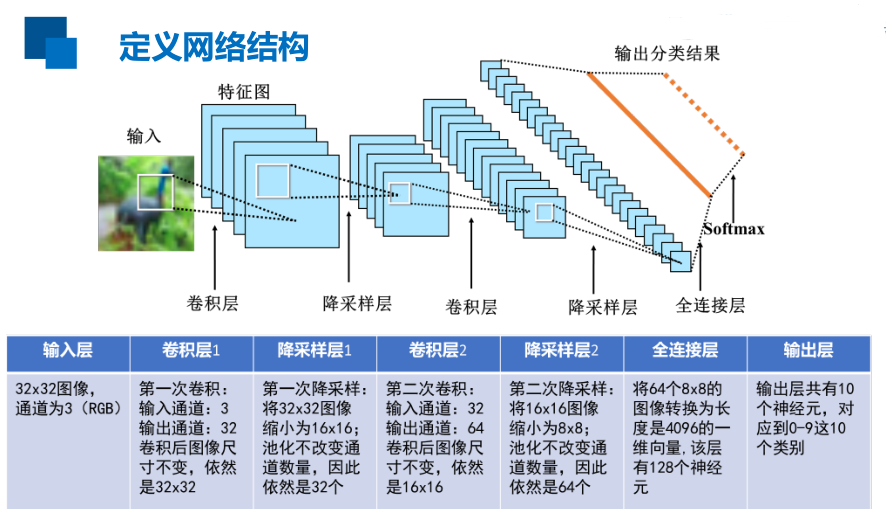
构建模型1
2
3
4
5
6
7
8
9
10
11
12with tf.name_scope("optimizer"):
#定义占位符
y = tf.placeholder("float", shape=[None,10],
name="label")
#定义损失函数
loss_function = tf.reduce_mean(
tf.nn.softmax_cross_entropy_with_logits_v2
(logits=pred,
labels=y))
#选择优化器
optimizer = tf.train.AdamOptimizer(learning_rate=0.0001)\
.minimize(loss_function)
定义准确率1
2
3
4with tf.name_scope("evaluation"):
correct_prediction = tf.equal(tf.argmax(pred,1),
tf.argmax(y,1))
accuracy = tf.reduce_mean(tf.cast(correct_prediction, "float"))
启动会话1
2
3
4
5
6
7
8
9
10
11
12
13
14import os
from time import time
train_epochs =25
batch_size = 50
total_batch = int(len(Xtrain)/batch_size)
epoch_list=[];accuracy_list=[];loss_list=[];
epoch = tf.Variable(0,name='epoch',trainable=False)
startTime=time()
sess = tf.Session()
init = tf.global_variables_initializer()
sess.run(init)
断点续训1
2
3
4
5
6
7
8
9
10
11
12
13
14
15
16#设置检查点存储目录
ckpt_dir = "CIFAR10_log"
if not os.path.exists(ckpt_dir):
os.makedirs(ckpt_dir)
#生成saver
saver = tf.train.Saver(max_to_keep=1)
#如果有检查点文件,读取最新的检查点文件,恢复各种变量值
ckpt = tf.train.latest_checkpoint(ckpt_dir )
if ckpt != None:
saver.restore(sess, ckpt)#力加载所有的参数
#从这里开始就可以直接使用模型进行预测,或者接着继续训练了
else:
print("Training from scratch.")
#获取续训参数
start = sess.run(epoch)
print("Training starts form {} epoch.".format(start+1))
迭代训练及改进1
2
3
4
5
6
7
8
9
10
11
12
13
14
15
16
17
18
19
20
21def get_train_batch(number, batch_size):
return Xtrain_normalize[number*batch_size:(number+1)*batch_size],\
Ytrain_onehot[number*batch_size:(number+1)*batch_size]
for ep in range(start, train_epochs):
for i in range(total_batch):
batch_x, batch_y = get_train_batch(i,batch_size)
sess.run(optimizer,feed_dict={x: batch_x, y: batch_y})
if i %100 == 0:
print("Step {}".format(i), "finished")
loss,acc = sess.run([loss_function,accuracy],feed_dict={x: batch_x, y: batch_y})
epoch_list.append(ep+1)
loss_list.append(loss);
accuracy_list.append(acc)
print("Train epoch:",'%02d'% (sess.run(epoch)+1),\
"Loss=","{:.6f}".format(loss),"Accuracy=",acc)
#保存检查点
saver.save(sess,ckpt_dir+".\CIFAR10_cnn_model.cpkt",global_step=ep+1)
sess.run(epoch.assign(ep+1))
duration =time()-startTime
print("Train finished takes: ",duration)
-增加网络层数
-增加迭代次数
-增加全连接层数
-增加全连接层的神经元个数
-数据扩增
可视化损失值1
2
3
4
5
6
7
8%matplotlib inline
import matplotlib.pyplot as plt
fig = plt.gcf()
fig.set_size_inches(4,2)
plt.plot(epoch_list, loss_list, label = 'loss')
plt.ylabel('loss')
plt.xlabel('epoch')
plt.legend(['loss'], loc='upper right')
可视化准确率1
2
3
4
5
6
7
8plt.plot(epoch_list, accuracy_list,label="accuracy" )
fig = plt.gcf()
fig.set_size_inches(4,2)
plt.ylim(0.1,1)
plt.ylabel('accuracy')
plt.xlabel('epoch')
plt.legend()
plt.show()
评估模型及预测1
2
3
4
5
6
7
8
9
10
11
12
13
14
15test_total_batch = int(len(Xtest_normalize)/batch_size)
test_acc_sum = 0.0
for i in range(test_total_batch):
test_image_batch = Xtest_normalize[i*batch_size:(i+1)*batch_size]
test_label_batch = Ytest_onehot[i*batch_size:(i+1)*batch_size]
test_batch_acc = sess.run(accuracy, feed_dict = {x:test_image_batch,y:test_label_batch})
test_acc_sum += test_batch_acc
test_acc = float(test_acc_sum/test_total_batch)
print("Test accuracy:{:.6f}".format(test_acc))
test_pred=sess.run(pred, feed_dict={x: Xtest_normalize[:10]})
prediction_result = sess.run(tf.argmax(test_pred,1))
plot_images_labels_prediction(Xtest, Ytest,prediction_result,0,10)
-计算测试集上的准确率
-利用模型进行预测
-可视化预测结果